使用 Perlin Noise、Catmull-Rom 创建闭合平滑曲线
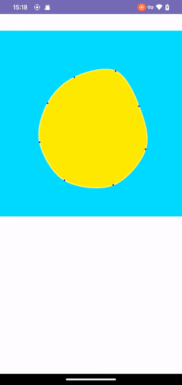
效果预览
前几天在 openprocessing 闲逛时,偶然发现了一个特别吸引我的动画效果——闭合的平滑曲线如同水波般优雅地流动变换。无独有偶,在一款白噪音助眠应用"潮汐"的界面中也看到过极为相似的设计语言,流畅的曲线随着声音节奏轻轻起伏,营造出令人放松的视觉效果。
最让我惊讶的是,这个即简约又充满韵律感的动画效果,核心代码竟然只有短短几行
function setup() { createCanvas(windowWidth, windowHeight);} function draw() { blendMode(BLEND); background(245); blendMode(MULTIPLY); noStroke(); translate(width/2,height/2); fill(255,150,0); drawLiq(8,100,80,200);} function drawLiq(vNnum,nm,sm,fcm){ push(); rotate(frameCount/fcm); let dr = TWO_PI/vNnum; beginShape(); for(let i = 0; i < vNnum + 3; i++){ let ind = i%vNnum; let rad = dr *ind; let r = height*0.3 + noise(frameCount/nm + ind) * height*0.1 + sin(frameCount/sm + ind)*height*0.05; curveVertex(cos(rad)*r, sin(rad)*r); } endShape(); pop();}而其中最关键的,是两个函数
- noise(Perlin noise):噪波函数
- curveVertex:Catmull-Rom 样条曲线
出于好奇,我试着去研究它们的实现原理,这个过程让我再次感受到,数学的魅力无处不在。
Perlin Noise
认识 Noise 函数
Perlin Noise(柏林噪声)是由计算机科学家 Ken Perlin 在 1983 年提出的一种梯度噪声算法。它能够生成自然、连续且随机的数值,广泛应用于计算机图形学、游戏开发和模拟自然现象(如地形、云层、火焰等)。与纯粹的随机噪声不同,Perlin Noise 具有平滑过渡的特性,使其更接近真实世界的自然纹理。
Perlin Noise 通过在空间中划分网格,并在每个网格节点上赋予随机梯度向量,然后通过插值计算出任意点的噪声值。这种算法能够在多次调用(相同的输入参数)时保持一致的数值,适合用于需要连续性和一致性的场景。
Perlin Noise 原理
Perlin Noise 的核心思想是通过插值使随机值平滑过渡。其实现步骤大致如下
- 网格定义:将空间划分为规则的网格,每个网格顶点分配一个随机梯度向量(单位向量)。
- 点积计算:对于空间中的任意一点,找到其所在网格的四个顶点,并计算该点到顶点的向量与顶点梯度向量的点积。
- 插值平滑:使用缓和曲线(如五次多项式)对四个顶点的点积结果进行双线性插值,确保噪声平滑过渡。
通过调整频率(网格密度)和叠加多层噪声(分形噪声),可以生成更复杂的自然效果。Perlin Noise 因其计算高效和自然表现,成为程序生成内容的重要工具。
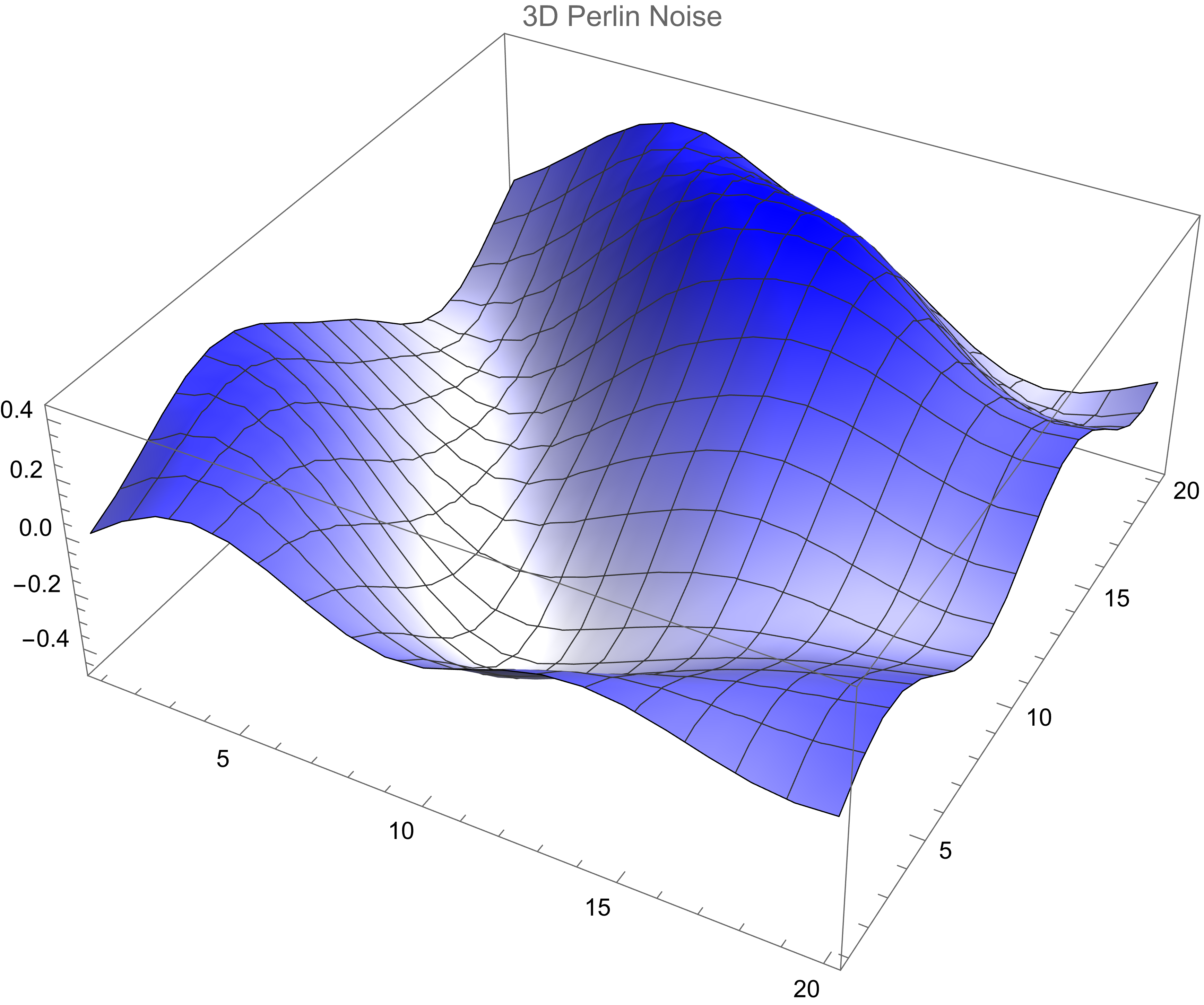
MatheMatica 演示 Perlin Noise 的计算
(* 1. 定义辅助函数 *)(* 生成随机单位向量 *)randomUnitVector := Normalize@RandomReal[{-1, 1}, 2] (* 生成梯度向量网格 *)generateGradientGrid[size_] := Table[randomUnitVector, {size}, {size}] (* 平滑插值函数 *)fade[t_] := 6 t^5 - 15 t^4 + 10 t^3;(* 线性插值 *)lerp[a_, b_, t_] := a + t*(b - a) (* 2. Perlin Noise 核心函数 *)perlinNoise2D[gradients_, x_, y_] := Module[{x0, y0, x1, y1, sx, sy, u, v, a, b}, (* 确定网格单元 *) x0 = Floor[x]; y0 = Floor[y]; x1 = x0 + 1; y1 = y0 + 1; (* 计算相对位置 *) sx = x - x0; sy = y - y0; (* 计算四个角点的贡献 *) u = dotProduct[gradients, x0, y0, x, y]; v = dotProduct[gradients, x1, y0, x, y]; a = lerp[u, v, fade[sx]]; u = dotProduct[gradients, x0, y1, x, y]; v = dotProduct[gradients, x1, y1, x, y]; b = lerp[u, v, fade[sx]]; lerp[a, b, fade[sy]]] (* 点积计算辅助函数 *)dotProduct[gradients_, ix_, iy_, x_, y_] := Module[{gradient, dx, dy}, gradient = gradients[[iy + 1, ix + 1]]; dx = x - ix; dy = y - iy; gradient . {dx, dy}] (* 3. 生成噪声图 *)(* 设置参数 *)(* 梯度网格大小 *)gridSize = 3;(* 噪声分辨率 *)noiseRes = 0.1;(* 生成梯度场 *)gradients = generateGradientGrid[gridSize]; (* 生成噪声数据 *)noiseData = Table[perlinNoise2D[gradients, x, y], {y, 0, gridSize - 1 - noiseRes, noiseRes}, {x, 0, gridSize - 1 - noiseRes, noiseRes}]; (* 4. 可视化 *)(* 自定义颜色函数:z 值小->白色,z 值大->蓝色 *)customColorFunction[z_] := Blend[{{0, White}, {1, Blue}}, z] (* 基本密度图 *)plot1 = ListDensityPlot[noiseData, ColorFunction -> customColorFunction, PlotRange -> All, ImageSize -> 500, PlotLabel -> "2D Perlin Noise"];(* 3D表面图 *)plot2 = ListPlot3D[noiseData, ColorFunction -> customColorFunction, PlotRange -> All, ImageSize -> 500, PlotLabel -> "3D Perlin Noise"];(* 并排显示 *)Row[{plot1, plot2}]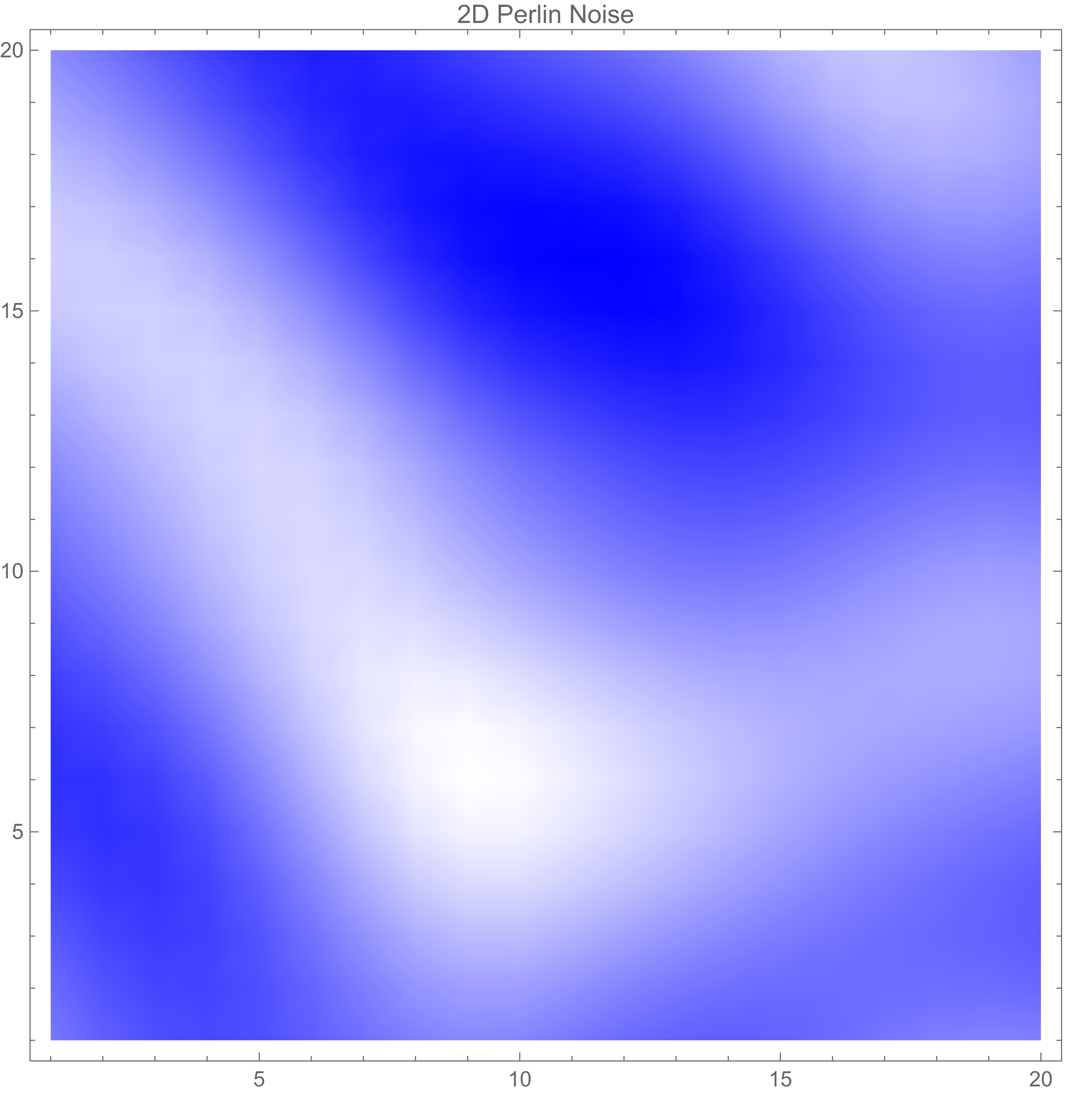
Catmull-Rom
认识 Catmull-Rom 样条曲线
Catmull-Rom 样条曲线是一种插值样条曲线,由 Edwin Catmull 和 Raphael Rom 提出。它能够平滑地穿过给定的控制点,适用于动画路径、相机轨迹和曲线拟合等场景。与 Bézier 曲线不同,Catmull-Rom 曲线保证经过每一个控制点,同时保持局部平滑性,使其在交互式设计中非常实用。
Catmull-Rom 样条曲线原理
Catmull-Rom 曲线的计算基于分段三次插值,其核心步骤如下:
- 局部控制:每四个相邻控制点(Pi−1,Pi,Pi+1,Pi+2)确定一段曲线,仅影响 Pi 到 Pi+1 之间的路径。
- 插值公式:使用 Hermite 插值形式,计算当前点 t∈[0,1] 的位置:
$$ P(t)=0.5⋅((2Pi)+(Pi+1−Pi−1)t+(2Pi−1−5Pi+4Pi+1−Pi+2)t2+(−Pi−1+3Pi−3Pi+1+Pi+2)t3) $$
- 张力参数(可选):可通过调整参数控制曲线的“紧度”,默认值为 0.5(均匀 Catmull-Rom 曲线)。
Catmull-Rom 曲线无需额外锚点,计算高效,且天然保持 C1 连续性,适合实时应用。
MatheMatica 演示 Catmull-Rom 样条曲线的计算
p0 = {1, 4};p1 = {3, 5};p2 = {4, 3};p3 = {6, 4};alpha = 0.5; (* 张力参数 *) t0 = 0;t1 = EuclideanDistance[p1, p0];t2 = t1 + EuclideanDistance[p2, p1] ^ alpha;t3 = t2 + EuclideanDistance[p3, p2] ^ alpha; CA1[t_] := ((t1 - t)/(t1 - t0)) * p0 + ((t - t0)/(t1 - t0)) * p1;CA2[t_] := ((t2 - t)/(t2 - t1)) * p1 + ((t - t1)/(t2 - t1)) * p2;CA3[t_] := ((t3 - t)/(t3 - t2)) * p2 + ((t - t2)/(t3 - t2)) * p3; CB1[t_] := ((t2 - t)/(t2 - t0)) * CA1[t] + ((t - t0)/(t2 - t0)) * CA2[t] ;CB2[t_] := ((t3 - t)/(t3 - t1)) * CA2[t] + ((t - t1)/(t3 - t1)) * CA3[t] ; CR[t_] := ((t2 - t)/(t2 - t1)) * CB1[t] + ((t - t1)/(t2 - t1)) * CB2[t]; Show[ ParametricPlot[ CA1[t], {t, 0, 6}, PlotStyle -> {Thin, Dashing[{0.01, 0.02}], Gray}, (* 红色虚线 *) PlotRange -> {{-1, 8}, {-1, 8}}, GridLines -> Automatic, GridLinesStyle -> LightGray, AxesLabel -> {"X", "Y"} ], ParametricPlot[ CA2[t], {t, 0, 6}, PlotStyle -> {Thick, Dashing[{0.01, 0.02}], Gray} (* 红色虚线 *) ], ParametricPlot[ CA3[t], {t, 0, 6}, PlotStyle -> {Thick, Dashing[{0.01, 0.02}], Gray} (* 红色虚线 *) ], ParametricPlot[ CB1[t], {t, 0, 6}, PlotStyle -> {Thick, Green} ], ParametricPlot[ CB2[t], {t, 0, 6}, PlotStyle -> {Thick, Green} ], ParametricPlot[ CR[t], {t, 0, 6}, PlotStyle -> {Thick, Red} ], Graphics[{ PointSize[0.02], Black, Point /@ {p0, p1, p2, p3}, Black, FontSize -> 12, Text["p0", p0, {0, 1.5}], Text["p1", p1, {0, 1.5}], Text["p2", p2, {0, 1.5}], Text["p3", p3, {0, 1.5}] }] ]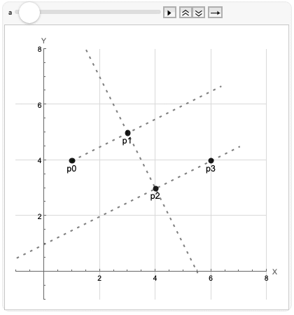
感兴趣的可以对比下 使用四段三次 Bézier 曲线拟合圆 中的贝塞尔曲线的计算示例图,同样四个点下不同的曲线表现
Android 中的实现
使用 Android 版的 Processing 开源框架
克隆源码 processing (android),主要使用其中的 processing-core 模块, 可在 module 下的 build.gradle 文件中引入
implementation project(':libs:processing-core')在 Activity 布局中添加 PFragment
class MainActivity : BaseActivity<ActivityMainBinding>(ActivityMainBinding::inflate){ override fun initViews() { super.initViews() val sketch = SketchBubble() val fragment = PFragment(sketch) fragment.setView(binding.flContent, this) }}SketchBubble 中即是具体的动画实现
package com.dafay.demo.lab.noise.processing import android.graphics.PointFimport com.dafay.demo.lib.base.utils.dp2pximport processing.core.PApplet class SketchBubble : PApplet() { private val pointList = mutableListOf<PointF>() override fun settings() { size(400.dp2px, 400.dp2px) } override fun setup() { hint(DISABLE_DEPTH_TEST) background(0f, 255f, 255f) } override fun draw() { // 绘制背景,覆盖上一帧的图像 background(0f, 255f, 255f) translate(width / 2f, height / 2f) rotate(frameCount.toFloat() / 500) drawBubble() } /** * 刷新 point */ private fun updatePointList() { pointList.clear() val dr = TWO_PI / 8.toFloat() for (i in 0 until 11) { val ind = i % 8 val rad = dr * ind val value1 = height * 0.3 val value2 = noise(frameCount / 500.toFloat() + ind) * height * 0.01 val value3 = sin(frameCount / 80.toFloat() + ind) * height * 0.05 val r = value1 + value2 + value3 val x = cos(rad) * r var y = sin(rad) * r pointList.add(PointF(x.toFloat(), y.toFloat())) } } private fun drawBubble() { stroke(255f, 255f, 125f) fill(255f, 255f, 0f) // 刷新点的位置 updatePointList() beginShape() pointList.forEach { // 绘制曲线 curveVertex(it.x, it.y) } endShape() // 绘制点 strokeWeight(PI * 3) stroke(0f, 0f, 255f) pointList.forEach { point(it.x, it.y) } }} 你可能会遇到的问题
processing (android) 中 curve 相关的绘制有个 bug ——无法清除之前的绘制,调试发现 path 没有进行重置,具体代码如下
// PGraphicsAndroid2D.java 文件public class PGraphicsAndroid2D extends PGraphics { static public boolean useBitmap = true; ... @Override protected void curveVertexSegment(float x1, float y1, float x2, float y2, float x3, float y3, float x4, float y4) { curveCoordX[0] = x1; curveCoordY[0] = y1; curveCoordX[1] = x2; curveCoordY[1] = y2; curveCoordX[2] = x3; curveCoordY[2] = y3; curveCoordX[3] = x4; curveCoordY[3] = y4; curveToBezierMatrix.mult(curveCoordX, curveDrawX); curveToBezierMatrix.mult(curveCoordY, curveDrawY); // since the paths are continuous, // only the first point needs the actual moveto if (vertexCount == 0) { // if (path == null) { // TODO: 这里添加一行代码,对路径进行重置 path.reset(); path.moveTo(curveDrawX[0], curveDrawY[0]); vertexCount = 1; } ...}/icons/cactus_gray.svg
创意编程还是直接使用 Processing JavaScript 更为高效。相比之下,使用 Android 进行开发不仅繁琐,还受到诸多限制,这让整个过程失去了不少乐趣。
自己动手实现
Android 可以使用自定义 View,覆盖 View::onDraw(),使用 Canvas 进行绘制
class BubbleView @JvmOverloads constructor(context: Context, attrs: AttributeSet? = null, defStyleAttr: Int = 0) : View(context, attrs, defStyleAttr) { // 画笔 private val paint = Paint().apply { style = Paint.Style.FILL_AND_STROKE strokeWidth = 6f color = Color.YELLOW isAntiAlias = true blendMode = BlendMode.SRC_OVER } // 噪声生成器 private val noiseGenerator = NoiseGenerator() // 绘制曲线 private val curveVertexRenderer = CurveVertexRenderer() private val pointList = mutableListOf<PointF>() private var frameCount = 0 private val vNum = 8 // 顶点数量 private val nm = 200f // 噪声参数 private val sm = 80f // 正弦参数 private val fcm = 15f // 旋转参数 private val animator = ValueAnimator.ofInt(0, Int.MAX_VALUE).apply { duration = Int.MAX_VALUE.toLong() repeatCount = ValueAnimator.INFINITE addUpdateListener { frameCount += 1 invalidate() } } override fun onAttachedToWindow() { super.onAttachedToWindow() animator.start() } override fun onDetachedFromWindow() { super.onDetachedFromWindow() animator.cancel() } override fun onDraw(canvas: Canvas) { super.onDraw(canvas) canvas.translate(width / 2f, height / 2f) canvas.rotate(frameCount.toFloat() / fcm) drawBubble(canvas) } /** * 刷新 point */ private fun updatePointList() { pointList.clear() val dr: Float = ((2 * PI) / vNum.toFloat()).toFloat() for (i in 0 until vNum + 3) { val ind: Int = i % vNum val rad: Float = dr * ind val value1 = height * 0.3 val value2 = noiseGenerator.noise(frameCount / nm + ind) * height * 0.01f val value3 = sin(frameCount / sm.toDouble() + ind) * height * 0.03f val r = (value1 + value2 + value3).toFloat() val x = cos(rad.toDouble()).toFloat() * r val y = sin(rad.toDouble()).toFloat() * r pointList.add(PointF(x, y)) } } fun drawBubble(canvas: Canvas) { updatePointList() paint.color = Color.YELLOW curveVertexRenderer.beginShape() pointList.forEach { curveVertexRenderer.curveVertex(it.x, it.y) } curveVertexRenderer.endShape(canvas, paint) paint.color = Color.BLUE pointList.forEach { canvas.drawCircle(it.x, it.y, 6f, paint) } } /** * 模拟 noise 函数 * 使用随机数模拟 noise 函数 */ class NoiseGenerator(private val seed: Int = 0) { private val permutation = IntArray(512).apply { val random = Random(seed.toLong()) val p = IntArray(256) { it } p.shuffle(random) for (i in 0 until 512) { this[i] = p[i and 255] } } private fun grad(hash: Int, x: Float): Float { val h = hash and 15 var grad = 1f + (h and 7) // 梯度值 1-8 if (h and 8 != 0) grad = -grad // 随机一半是负数 return grad * x } fun noise(x: Float): Float { val xi = x.toInt() and 255 val xf = x - x.toInt() val u = fade(xf) val a = permutation[xi] val b = permutation[xi + 1] return lerp(u, grad(a, xf), grad(b, xf - 1f)) * 0.5f + 0.5f } private fun fade(t: Float): Float = t * t * t * (t * (t * 6f - 15f) + 10f) private fun lerp(amount: Float, a: Float, b: Float) = a + amount * (b - a) } /** * Catmull-Rom 样条曲线绘制 */ class CurveVertexRenderer { private val points: MutableList<PointF> = ArrayList() // p1,p2 之间有多少点,点越多曲线越平滑 private val diff = 0.1f fun beginShape() { points.clear() } /** * 收集所有参与绘制的点 */ fun curveVertex(x: Float, y: Float) { points.add(PointF(x, y)) } /** * 执行绘制 */ fun endShape(canvas: Canvas, paint: Paint) { if (points.size < 4) { return // 至少需要4个点才能生成曲线 } val path = Path() for (i in 0..points.size - 4) { val p0 = points[i] val p1 = points[i + 1] val p2 = points[i + 2] val p3 = points[i + 3] for (i in 0..(1/diff).toInt()) { if (i == 0) { path.lineTo(p1.x, p1.y) } val point = catmullRomInterpolation(p0, p1, p2, p3, i*diff) path.lineTo(point.x, point.y) } } canvas.drawPath(path, paint) } /** * catmull-rom 计算,张力默认 0.5 */ fun catmullRomInterpolation( p0: PointF, // 前一个点 p1: PointF, // 起点 p2: PointF, // 终点 p3: PointF, // 后一个点 t: Float // 插值参数 [0,1] ): PointF { // 计算 x 坐标 val x = 0.5f * ( (2 * p1.x) + (-p0.x + p2.x) * t + (2 * p0.x - 5 * p1.x + 4 * p2.x - p3.x) * t * t + (-p0.x + 3 * p1.x - 3 * p2.x + p3.x) * t * t * t ) // 计算 y 坐标 val y = 0.5f * ( (2 * p1.y) + (-p0.y + p2.y) * t + (2 * p0.y - 5 * p1.y + 4 * p2.y - p3.y) * t * t + (-p0.y + 3 * p1.y - 3 * p2.y + p3.y) * t * t * t ) return PointF(x, y) } }} 